The objective of this lab is to enhance understanding of limit evaluation techniques, particularly focusing on factoring, multiplying by a smart one, and using symbolic computation tools such as Maxima to solve problems involving limits. Students will:
Learn to Factor to Cancel Terms:
Understand the process of factoring expressions to cancel terms in limit problems.
Use Maxima to factor and simplify expressions, and observe the impact on limit calculations.
Analyze the plot of the function to gain insights into the behavior of the limit.
Practice Multiplying by a Smart One:
Learn how multiplying by a conjugate can help simplify and evaluate limits.
Use Maxima to perform these multiplications and simplify the expressions.
Plot the function to visually interpret the behavior of the limit.
Explore the Concept of (e):
Calculate the slopes of secant lines as they approach the tangent line for exponential functions with different bases.
Use Maxima to compute and display these slopes, and analyze the results.
Understand the relationship between the slopes of secant lines, the natural logarithm, and the number \(e\).
Apply the Squeeze Theorem:
Plot functions that bound another function to use the squeeze theorem.
Use Maxima to compute limits and verify the conclusions drawn from the squeeze theorem.
Evaluate Trigonometric Limits:
Use Maxima to calculate specific trigonometric limits.
Explain the steps involved in solving these limits manually to reinforce understanding.
Develop Problem-Solving Skills:
Complete and answer questions throughout the lab, using the knowledge and techniques learned.
Solve similar problems by hand and verify the results using Maxima.
By the end of this lab, students will have a solid grasp of various limit evaluation techniques, proficiency in using Maxima for symbolic computation, and improved problem-solving skills for limits and related concepts.
Using the formatting of reporting learned on the last lab, follow the explanations, and complete all the questions (Q:) on each section.
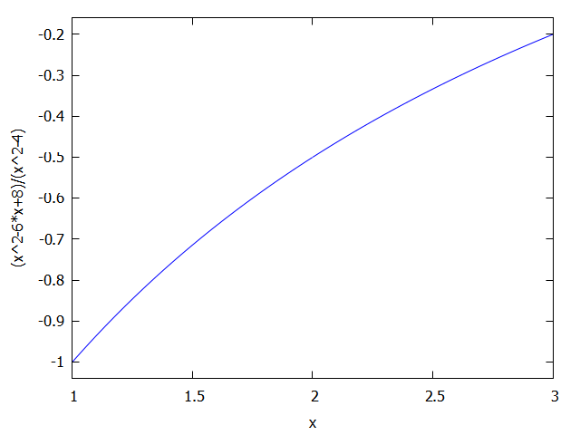
Maxima is strong! can calculate the limits for you very easily1:
(%i11) limit(y(x),x,1);
(%o11) 1/2
(%i12) plot2d(y(x),[x,0,2]);
2.2.3Q: Observing the plot, what you can comment about the limit?
2.3 What is \(e\)?
If we calculate the slope of the secant line as the two points get closer to each other, we understand that converge to the slope of the tangent line for a single point.
\[\lim_{\Delta x \rightarrow 0} m_{sec} = m_{tan}\]
Now, if we have an exponential of base 2, \(2^x\), and we calculate the convergence of the secant line to the tangent line at \(x=0\) we observe that:
\[\boxed{f(x)=2^x}\]
/* Define the function f(x) */f(x) := 2^x;/* Define the msec function */define(msec(x1, x2), (f(x2) - f(x1)) / (x2 - x1));/* List of specific values */val: [2, 1, 0.5, 0.1, 0.01, 0.001];/* Loop to evaluate msec(0, i) for each value in the list */foriinvaldo (display(msec(0, i)));
2.3.1Q: After running this script, explain what it does. As the two points get closer what happen with the slope of the secant?
\[\boxed{f(x)=3^x}\]
/* Define the function f(x) */f(x) := 3^x;/* Define the msec function */define(msec(x1, x2), (f(x2) - f(x1)) / (x2 - x1));/* List of specific values */val: [2, 1, 0.5, 0.1, 0.01, 0.001];/* Loop to evaluate msec(0, i) for each value in the list */foriinvaldo (display(msec(0, i)));
2.3.2Q: After running this script, explain what it does. As the two points get closer what happen with the slope of the secant?
\[\boxed{f(x)=4^x}\]
/* Define the function f(x) */f(x) := 4^x;/* Define the msec function */define(msec(x1, x2), (f(x2) - f(x1)) / (x2 - x1));/* List of specific values */val: [2, 1, 0.5, 0.1, 0.01, 0.001];/* Loop to evaluate msec(0, i) for each value in the list */foriinvaldo (display(msec(0, i)));
2.3.3Q: After running this script, explain what it does. As the two points get closer what happen with the slope of the secant?
2.3.4Q: Using maxima calculate \(\log(2)\), \(\log(3)\), and \(\log(4)\)
(%i13) log(2),numer;
(%o13) 0.6931471805599453
(%i14) log(3),numer;
(%o14) 1.0986122886681098
(%i15) log(4),numer;
(%o15) 1.3862943611198906
2.3.5Q: How this 3 quantities relate with the slopes of the secant we calculated before?
2.3.6Q: What you can conclude about the slopes of any exponential at \(x=0\)?
2.3.7Q: What is the definition of \(e\) ?
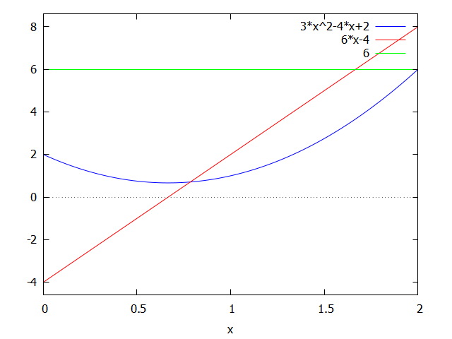
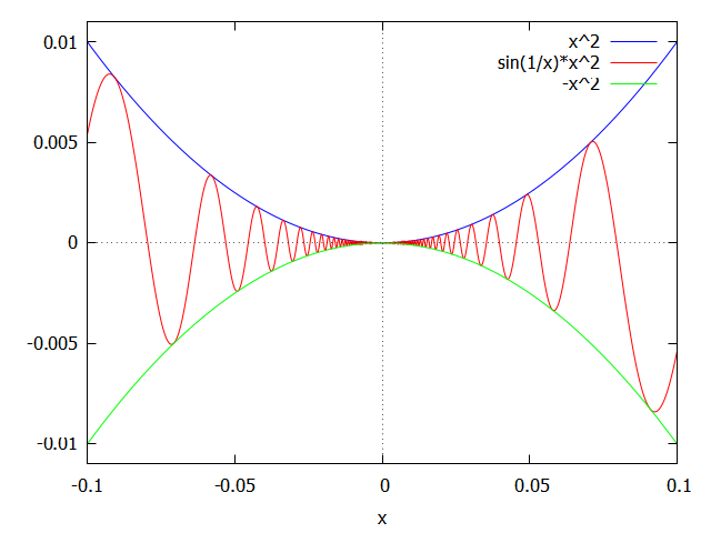
2.4 The squeeze theorem
Assume the functions \(f,g,\text{ and }h\) satisfy \(f(x)\leq g(x) \leq h(x)\) for all values of \(x\) near \(a\), except possibly at \(a\).
If \[\lim_{x\rightarrow a} f(x)=\lim_{x\rightarrow a} h(x)=L\], then \[\lim_{x\rightarrow a} g(x) =L\]
2.4.1 Plot the following functions on the same window
2.5.2Q:Explain how you will solve the same problem by hand
Answer here:
2.6 For each of the previous sections:
take a picture of your handwritten work, submit them to the dropbox, and then also linked to the corresponding section of your wxmaxima document2 (Cell -> Insert Image)
be sure your code run correctly by pressing Shift+Enter in each code chunk.
be sure the whole document display correctly, by running Ctrl+R
Submit on the corresponding Dropbox folder, with the corresponding name (FINAL_Lab2_Calc1_YOURLASTNAME_mmddyy.wxmx.)
Exams are handwritten, so you still need to learn the techniques, but using computation you can get insights and learn better↩︎
pictures need to be in the same folder of your .wxmx file↩︎